1 Statistical Summary Tables

1.1 Introduction.

Till now, you have been exploring and understanding datasets. After EDA, the analysis phase is undertaken wherein you need to look carefully at associations between the outcome and exposure variables, in other words, independent and dependent variables. There can be two variables wherein you are interested in associations such as independent sample t-tests for difference between means, or a Chi-square test, or paired test, etc depending on the variables and Research Questions.

In this session, we shall take you through some commonly used tests and their presentation tables including basics of regression models.

1.2 Inferential statistics: An overview

1.2.1 Is birth weight associated with Maternal factors?

For this question, the summary statistics should be split by birth weight categories, which can be done by using the by= argument. To compare two or more groups, include add_p() with the function call, which detects variable type and uses an appropriate statistical test.

Caution

The tbl_summary() provides outputs and inferential statistics according to computed distribution. It is important to consider which test to apply and when.. discuss!!

Code
df |> 
  select(-smoke,
         -race) |> 
  tbl_summary(
    statistic = all_continuous() ~ "{mean}, {sd}",
    label = list(maternal_weight ~ "Maternal Weight",
                 maternal_age ~ "Maternal Age",
                 smoke_cat ~ "Smoking History"),
    by = child_weight_cat
  ) |> 
  add_p()
Characteristic Normal, N = 1301 Low Birth Weight, N = 591 p-value2
Maternal Age 23.7, 5.6 22.3, 4.5 0.2
Maternal Weight 133, 32 122, 27 0.013
number_preterm <0.001
    0 118 (91%) 41 (69%)
    1 8 (6.2%) 16 (27%)
    2 3 (2.3%) 2 (3.4%)
    3 1 (0.8%) 0 (0%)
hypertension 5 (3.8%) 7 (12%) 0.052
uterine_irritability 14 (11%) 14 (24%) 0.020
health_visits 0.3
    0 64 (49%) 36 (61%)
    1 36 (28%) 11 (19%)
    2 23 (18%) 7 (12%)
    3 3 (2.3%) 4 (6.8%)
    4 3 (2.3%) 1 (1.7%)
    6 1 (0.8%) 0 (0%)
birth_weight 3,329, 478 2,097, 391 <0.001
Smoking History 0.026
    Non-smoker 86 (66%) 29 (49%)
    Smoker 44 (34%) 30 (51%)
race_cat 0.082
    White 73 (56%) 23 (39%)
    Black 15 (12%) 11 (19%)
    Other 42 (32%) 25 (42%)
1 Mean, SD; n (%)
2 Wilcoxon rank sum test; Fisher’s exact test; Pearson’s Chi-squared test

1.2.2 Specifying which test to apply

Code
df |> 
  select(-smoke,
         -race) |> 
  tbl_summary(
    statistic = all_continuous() ~ "{mean}, {sd}",
    label = list(maternal_weight ~ "Maternal Weight",
                 maternal_age ~ "Maternal Age",
                 smoke_cat ~ "Smoking History"),
    by = child_weight_cat
  ) |> 
  add_p(all_continuous() ~ "t.test")
Characteristic Normal, N = 1301 Low Birth Weight, N = 591 p-value2
Maternal Age 23.7, 5.6 22.3, 4.5 0.078
Maternal Weight 133, 32 122, 27 0.013
number_preterm <0.001
    0 118 (91%) 41 (69%)
    1 8 (6.2%) 16 (27%)
    2 3 (2.3%) 2 (3.4%)
    3 1 (0.8%) 0 (0%)
hypertension 5 (3.8%) 7 (12%) 0.052
uterine_irritability 14 (11%) 14 (24%) 0.020
health_visits 0.3
    0 64 (49%) 36 (61%)
    1 36 (28%) 11 (19%)
    2 23 (18%) 7 (12%)
    3 3 (2.3%) 4 (6.8%)
    4 3 (2.3%) 1 (1.7%)
    6 1 (0.8%) 0 (0%)
birth_weight 3,329, 478 2,097, 391 <0.001
Smoking History 0.026
    Non-smoker 86 (66%) 29 (49%)
    Smoker 44 (34%) 30 (51%)
race_cat 0.082
    White 73 (56%) 23 (39%)
    Black 15 (12%) 11 (19%)
    Other 42 (32%) 25 (42%)
1 Mean, SD; n (%)
2 Welch Two Sample t-test; Fisher’s exact test; Pearson’s Chi-squared test

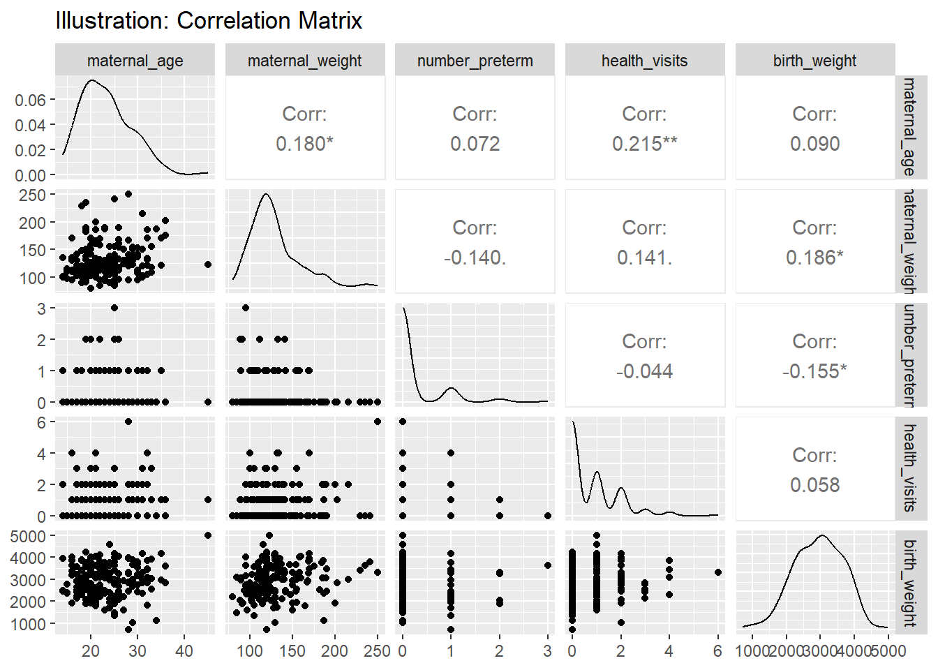
1.3 Correlation matrices

Example. As a researcher, you might be interested in knowing the correlation between maternal weight, number of preterm births, number of health visits and child birth weight.

Code
GGally::ggpairs(df |> 
          select(maternal_age, maternal_weight,
                 number_preterm, health_visits,
                 birth_weight),
        title="Illustration: Correlation Matrix") 

1.4 Regression analysis tables

The tbl_regression() function takes a regression model object in R and returns a formatted table of regression model results that is publication-ready. It is a simple way to summarize and present your analysis results using R! Like tbl_summary(), tbl_regression() creates highly customizable analytic tables with sensible defaults.

Code
# build logistic regression model
m1 <- glm(child_weight_cat ~ maternal_age + smoke_cat, 
          data = df, 
          family = binomial)

# view raw model results
summary(m1)$coefficients
                   Estimate Std. Error     z value   Pr(>|z|)
(Intercept)      0.06090554 0.75731970  0.08042249 0.93590124
maternal_age    -0.04977927 0.03197195 -1.55696724 0.11947826
smoke_catSmoker  0.69184868 0.32180606  2.14989327 0.03156366
Code
# Create presentation table
tbl_regression(m1, exponentiate = TRUE)
Characteristic OR1 95% CI1 p-value
maternal_age 0.95 0.89, 1.01 0.12
smoke_cat
    Non-smoker
    Smoker 2.00 1.06, 3.77 0.032
1 OR = Odds Ratio, CI = Confidence Interval

1.5 Summary.

In this section, we have introduced you to creating presentable tables for inferential statistics, correlation, and regression tables. Considering time, we are not dwelling deep into which test to apply and when concept. Rather we have focused on how to do them. It is strongly recommended to use these powerful tools in consultation with a Statistician/ Epidemiologist for meaningful inferences and robust methodologies. Hope you had an enjoyable learning during the sessions and we could answer your queries and show you additional resources during the workshop. Be in touch…Happy Learning!