Exploratory Time Series Analysis

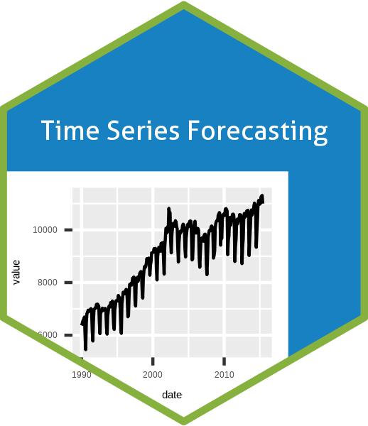
Welcome to the world of Time Series Analysis and forecasting!!

1 Introduction.

In this section, we shall be discussing about exploratory data analysis concepts specific to time series analysis. It is important to note that traditional statistical approach such as calculating measures of central tendencies and measures of dispersion remains an integral part of any analysis, however, we shall be looking at them during workshop exercises and not here.

2 Concept of stationarity and transformations.

It is important to understand that ARIMA models are based on assumption that the time series data is stationary in nature. A time series is said to be stationary when the mean value of each time component is similar (i.e no trend or seasonality). In other words, A stationary time series is one whose statistical properties do not depend on the time at which the series is observed. However, often that is not the case. If the data shows variation that increases or decreases with the level of the series, then a transformation can be useful. For example, a logarithmic transformation is often useful to make a series stationary. Another useful family of transformations, that includes both logarithms and power transformations, is the family of Box-Cox transformations. Also, differencing of the order one or two is a commonly used approach for making time series stationary. We shall be discussing this topic further as we progress in the workshop for a better understanding.

3 Time series components.

A time series data is often described in terms of trend, seasonality and cyclicity.

• Trend. A trend is said to be present when there is a long-term increase or decrease in the data. This change does not always have to be linear.

• Seasonality. A seasonal pattern occurs when a time series is affected by seasonal factors such as the time of the year or the day of the week. Seasonality is always of a fixed and known period.

• Cyclicity. A cycle occurs when the data exhibit rises and falls that are not of a fixed frequency.

4 Visualizations.

4.1 Time plots

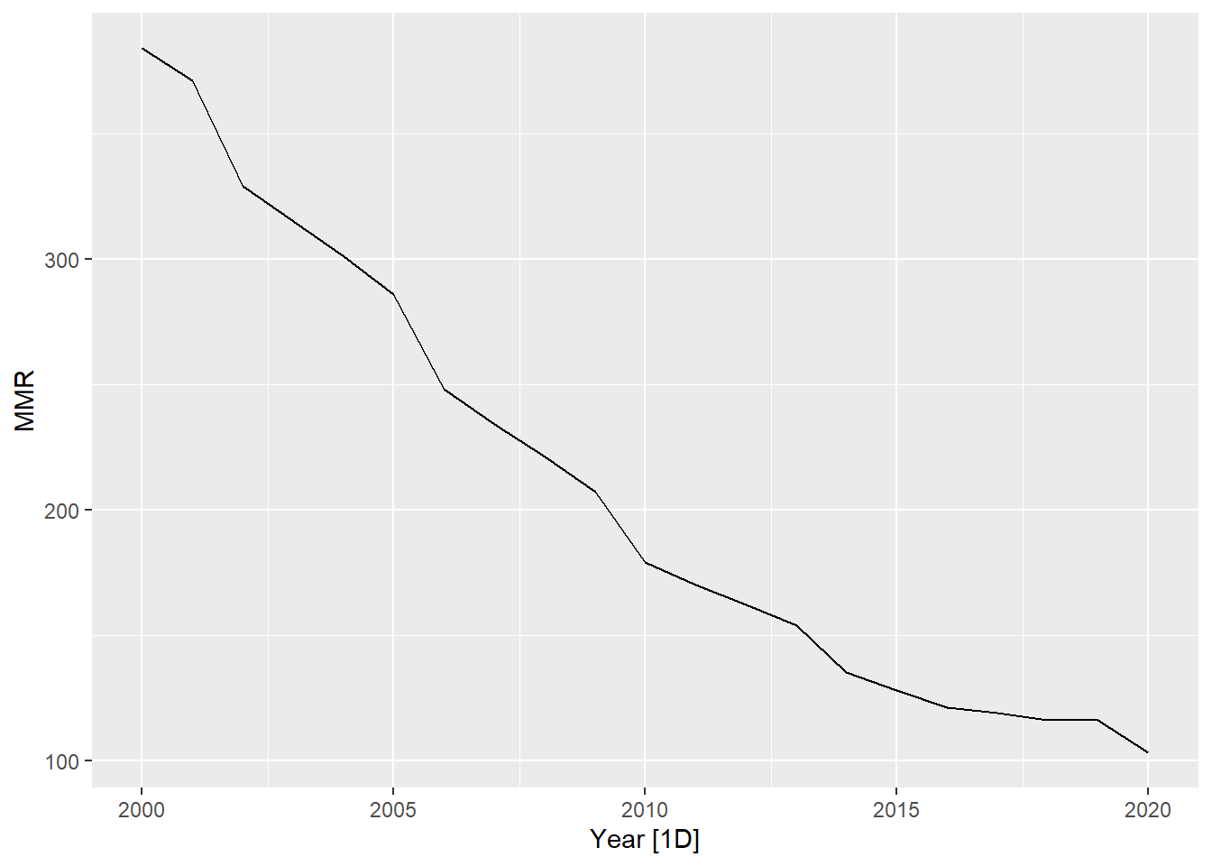
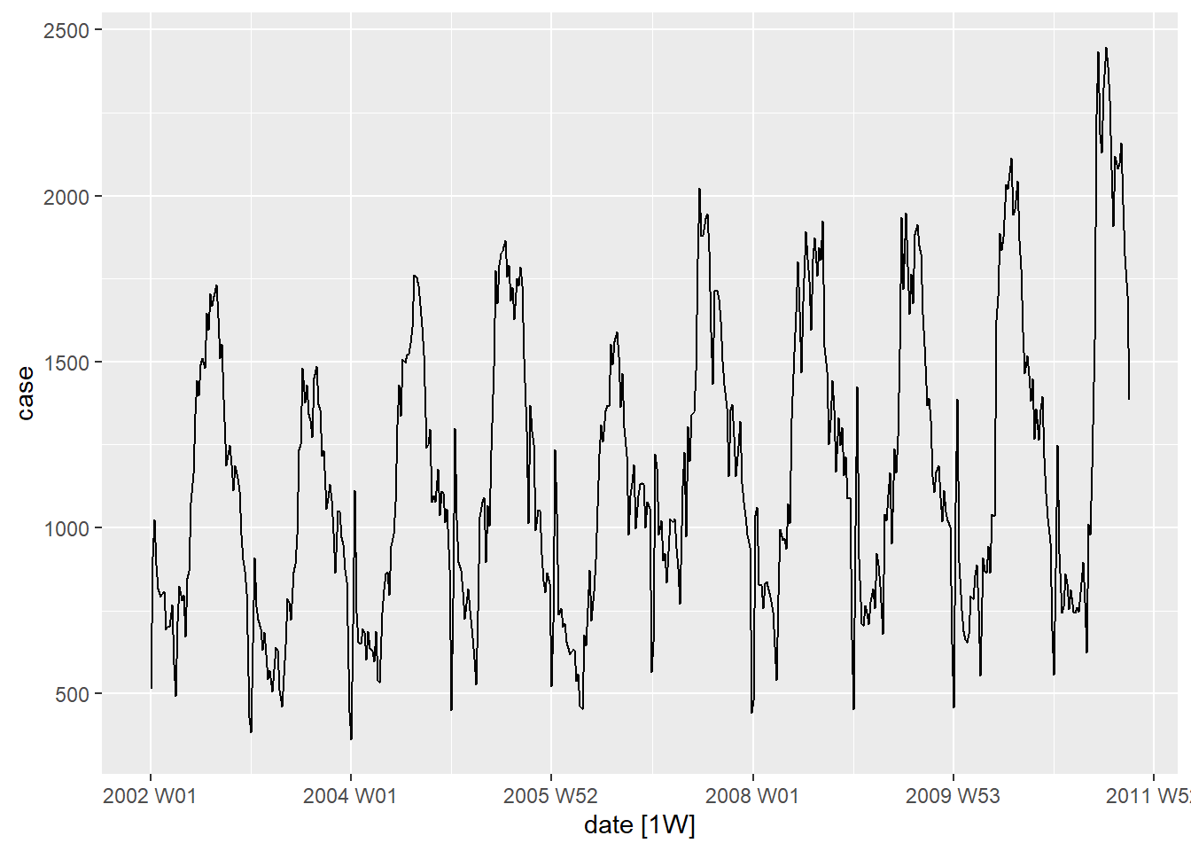
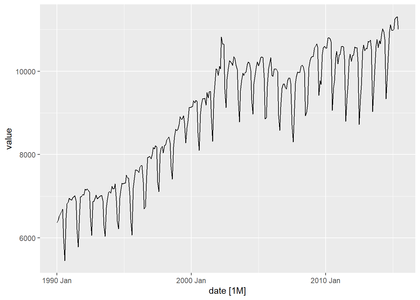
What kind of trend, seasonality and cyclicity do you observe in the following visualizations?

# Creating tsibble objects

df_aqi <- df_aqi |> 
  as_tsibble() 

Using `Sample Date` as index variable.

df_rta <- df_rta |> 
  as_tsibble() 

df_disaster <- df_disaster |> 
  as_tsibble() 

df_mmr <- df_mmr |> 
  mutate(Year = dmy(
    str_c("01-01-", Year)
  )) |> 
  as_tsibble() 

Using `Year` as index variable.

df_campylo <- df_campylo |> 
  mutate(date = yearweek(date)) |> 
  as_tsibble() 

Using `date` as index variable.

df_750 <- df_750 |> 
  mutate(date = yearmonth(date)) |> 
  as_tsibble() 

Using `date` as index variable.

Code

df_aqi |> 
  autoplot()
df_rta |> 
  autoplot()
df_disaster |> 
  autoplot()
df_mmr |> 
  autoplot()
df_campylo |> 
  autoplot()
df_750 |> 
  autoplot()
df_diab |> 
  autoplot()

(a) AQI

(b) RTA

(c) Earthquakes

(d) MMR

(e) Campylobacter

(f) M750

(g) Diabetes drug sales

Figure 1: Visualizations for Trend, seasonality and cyclicity

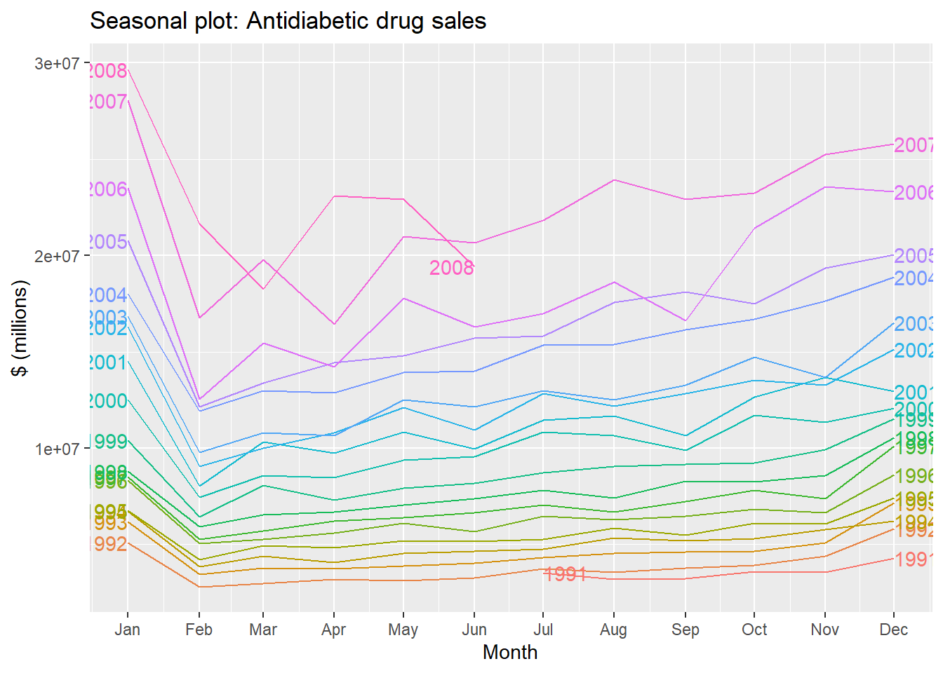
4.2 Seasonal plots.

A seasonal plot is similar to a time plot except that the data are plotted against the individual “seasons” in which the data were observed.A seasonal plot allows the underlying seasonal pattern to be seen more clearly, and is especially useful in identifying years in which the pattern changes.

df_diab |>
  gg_season(TotalC, labels = "both") +
  labs(y = "$ (millions)",
       title = "Seasonal plot: Antidiabetic drug sales")

4.3 Seasonal subseries plot.

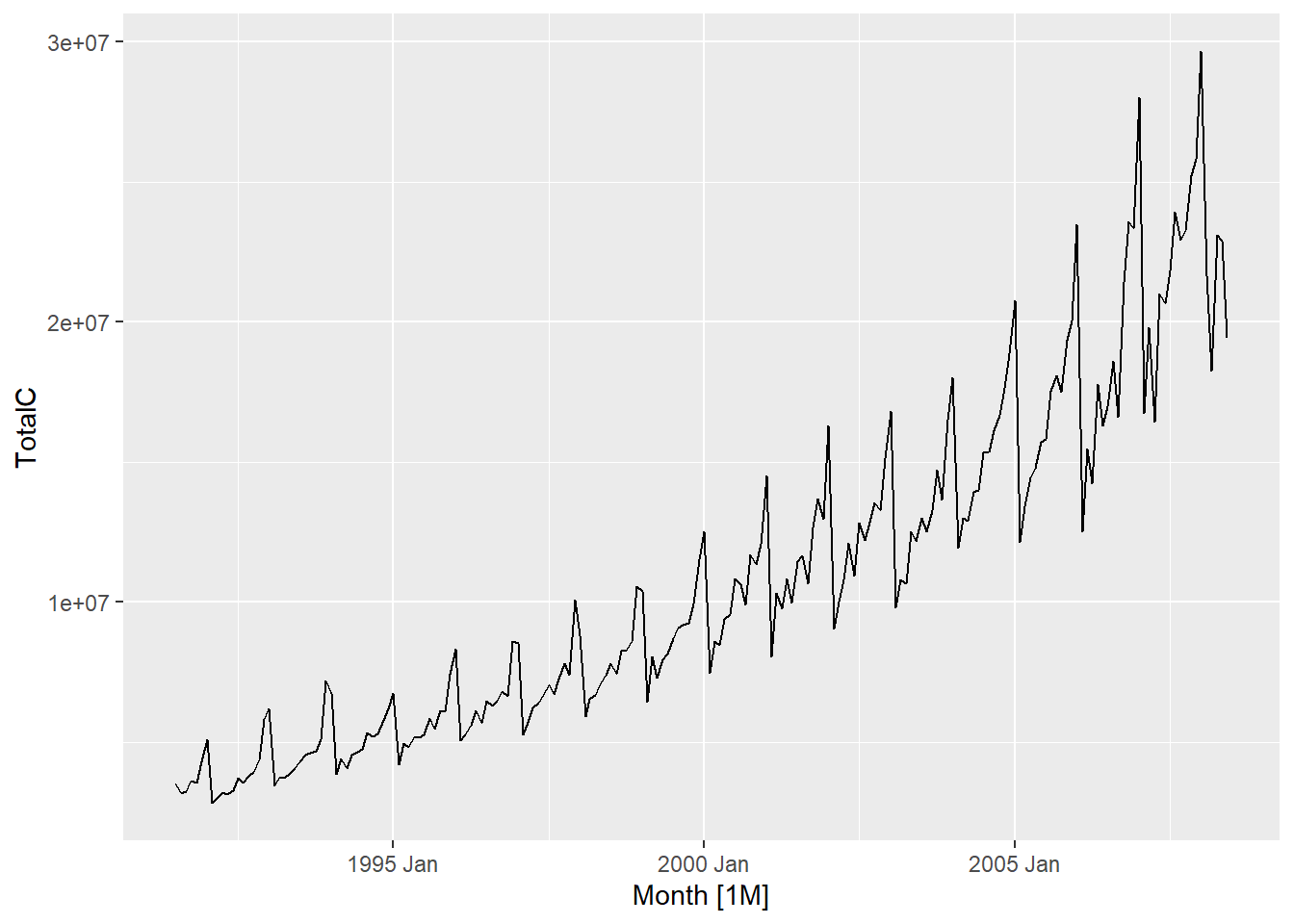
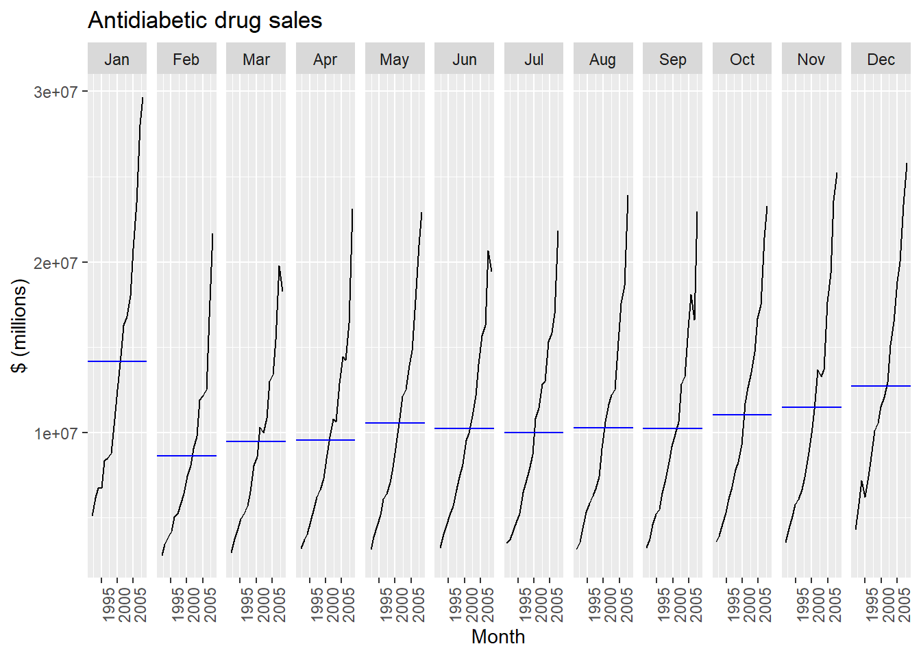
Seasonal subseries plot is an alternative plot that emphasises the seasonal patterns is where the data for each season are collected together in separate mini time plots. The blue horizontal lines indicate the means for each month. This form of plot enables the underlying seasonal pattern to be seen clearly, and also shows the changes in seasonality over time. It is especially useful in identifying changes within particular seasons.

df_diab |>
  gg_subseries(TotalC) +
  labs(
    y = "$ (millions)",
    title = "Antidiabetic drug sales"
  )

5 Time series features.

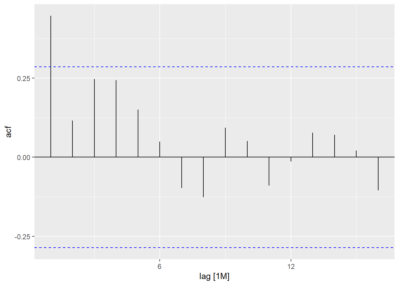
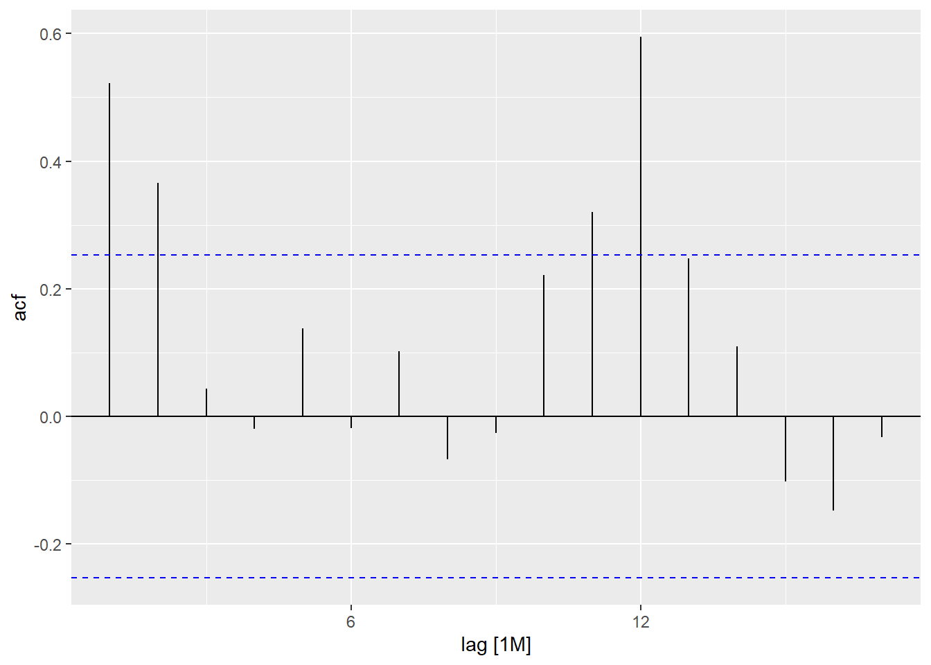
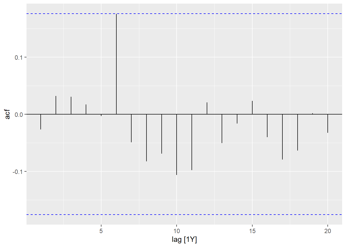
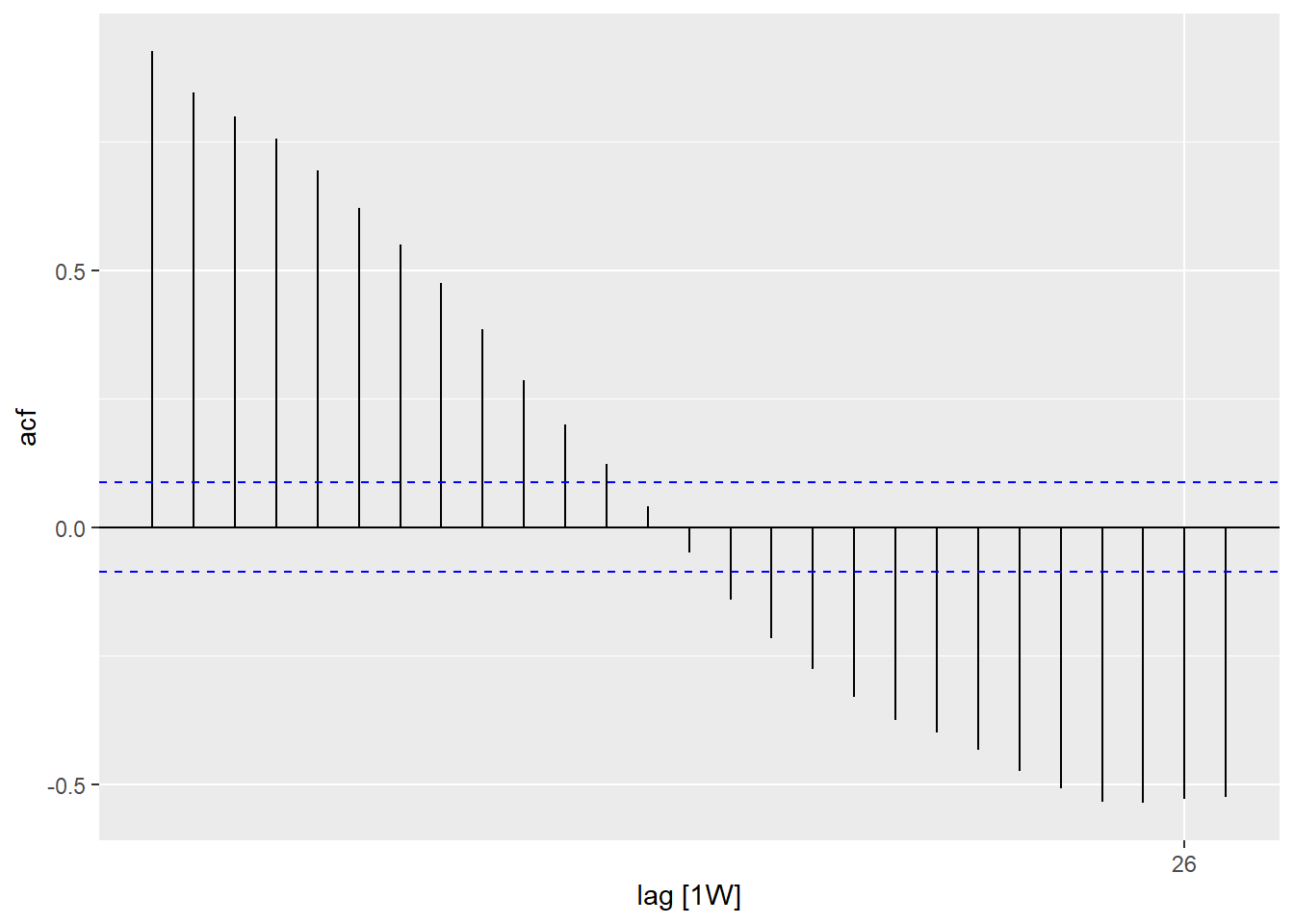
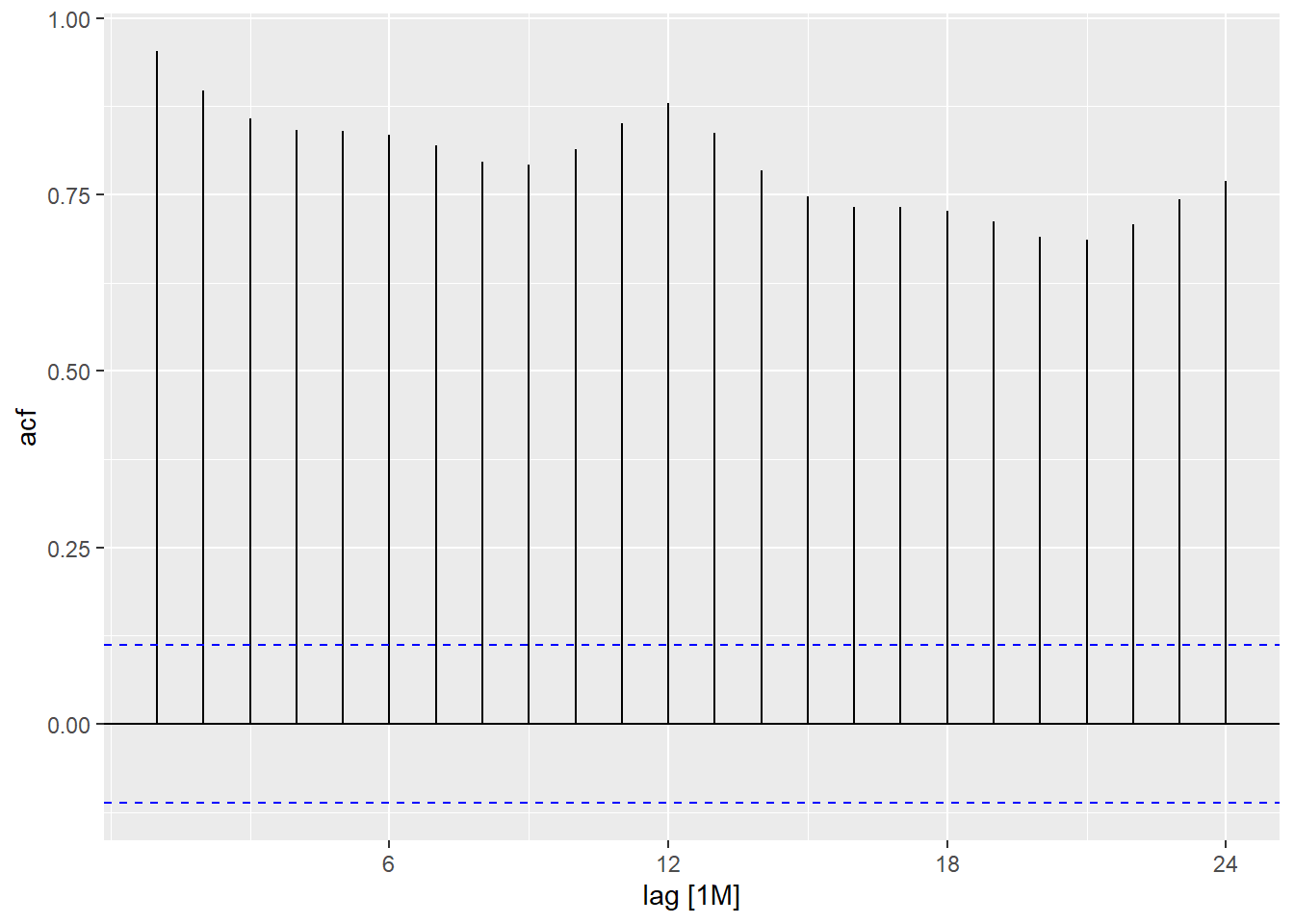
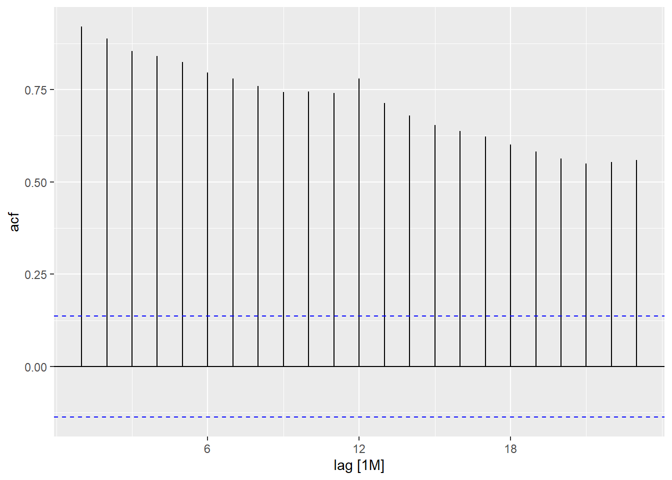
5.1 Autocorrelation function (ACF)

Just as correlation measures the extent of a linear relationship between two variables, autocorrelation measures the linear relationship between lagged values of a time series. In a time series, the autocorrelation coefficients between varied lags make up the autocorrelation function or ACF.

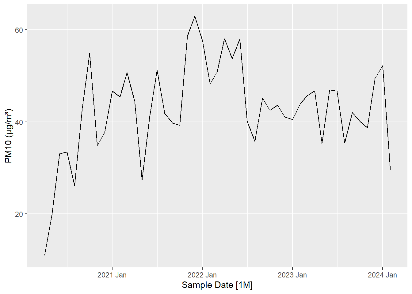
df_aqi |> 
  ACF(`PM10 (µg/m³)`, 
      lag_max = 5)

# A tsibble: 5 x 2 [1M]
       lag   acf
  <cf_lag> <dbl>
1       1M 0.447
2       2M 0.116
3       3M 0.247
4       4M 0.244
5       5M 0.150

The same can also be visualized through ACF plot for better understanding.

Code

df_aqi |> 
  ACF(`PM10 (µg/m³)`) |> 
  autoplot()
df_rta |> 
  ACF(accidents) |> 
  autoplot()
df_disaster |> 
  ACF(deaths_earthquakes) |> 
  autoplot()
df_campylo |> 
  ACF(case) |> 
  autoplot()
df_750 |> 
  ACF(value) |> 
  autoplot()
df_diab |> 
  ACF(TotalC) |> 
  autoplot()

(a) AQI

(b) RTA

(c) Earthquakes

(d) MMR

(e) Campylobacter

(f) M750

Figure 2: Visualizations for Trend, seasonality and cyclicity

5.2 Additional ACF features

The feat_acf() function computes a selection of the autocorrelations as under:

• The first autocorrelation coefficient from the original data; the sum of squares of the first ten autocorrelation coefficients from the original data;
• The first autocorrelation coefficient from the differenced data;
• The sum of squares of the first ten autocorrelation coefficients from the differenced data;
• The first autocorrelation coefficient from the twice differenced data;
• The sum of squares of the first ten autocorrelation coefficients from the twice differenced data;
• For seasonal data, the autocorrelation coefficient at the first seasonal lag is also returned.

Code

df_aqi |>
  features(`PM10 (µg/m³)`,
           feat_acf)|> 
  pivot_longer(cols = everything())

# A tibble: 7 × 2
  name          value
  <chr>         <dbl>
1 acf1         0.447 
2 acf10        0.395 
3 diff1_acf1  -0.121 
4 diff1_acf10  0.540 
5 diff2_acf1  -0.318 
6 diff2_acf10  0.599 
7 season_acf1 -0.0140

6 Time series decomposition

Decomposition methods

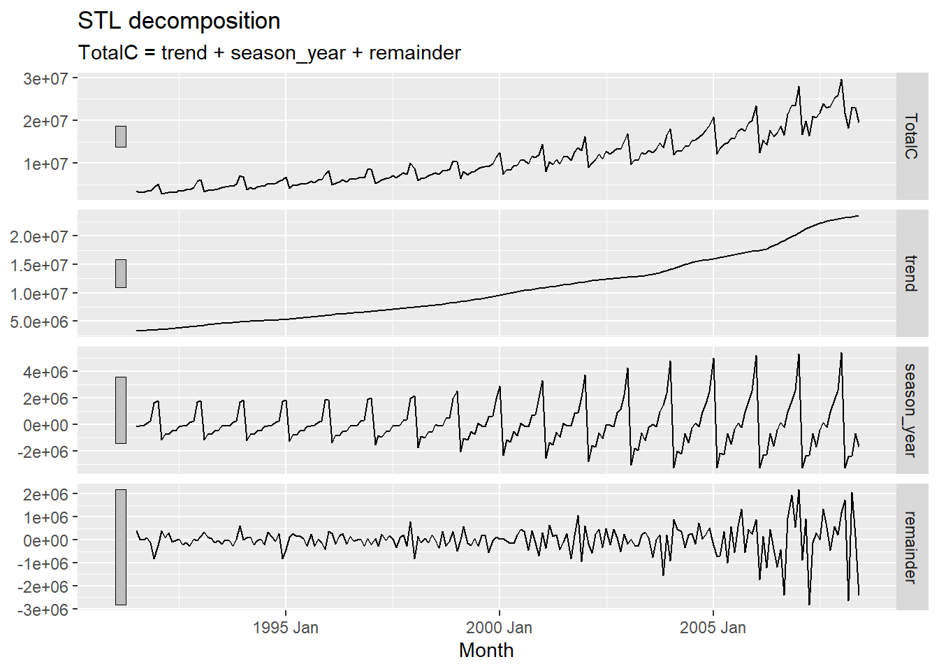
The additive decomposition is the most appropriate if the magnitude of the seasonal fluctuations, or the variation around the trend-cycle, does not vary with the level of the time series. When the variation in the seasonal pattern, or the variation around the trend-cycle, appears to be proportional to the level of the time series, then a multiplicative decomposition is more appropriate.

Time series data is decomposed into trend, seasonality and remainder components based on additive or multiplicative decomposition methods. If we assume an additive decomposition, then we can write \(y_t = S_t + T_t + R_t\) where \(y_t\) is the data, \(S_t\) is the seasonal component, \(T_t\) is the trend-cycle component, and \(R_t\) is the remainder component, all at period \(t\). Alternatively, a multiplicative decomposition would be written as \(y_t = S_t * T_t * R_t\).

df_diab |>
  model(stl = STL(TotalC)) |> 
  components()

# A dable: 204 x 7 [1M]
# Key:     .model [1]
# :        TotalC = trend + season_year + remainder
   .model    Month  TotalC    trend season_year remainder season_adjust
   <chr>     <mth>   <dbl>    <dbl>       <dbl>     <dbl>         <dbl>
 1 stl    1991 Jul 3526591 3270635.    -127065.   383021.      3653656.
 2 stl    1991 Aug 3180891 3310236.    -116422.   -12923.      3297313.
 3 stl    1991 Sep 3252221 3349837.     -87179.   -10437.      3339400.
 4 stl    1991 Oct 3611003 3389438.     134369.    87196.      3476634.
 5 stl    1991 Nov 3565869 3429518.     254173.  -117822.      3311696.
 6 stl    1991 Dec 4306371 3469598.    1640931.  -804158.      2665440.
 7 stl    1992 Jan 5088335 3509677.    1811795.  -233137.      3276540.
 8 stl    1992 Feb 2814520 3549836.   -1143268.   407952.      3957788.
 9 stl    1992 Mar 2985811 3589994.    -704096.    99913.      3689907.
10 stl    1992 Apr 3204780 3630153.    -727385.   302012.      3932165.
# ℹ 194 more rows

df_diab |>
  model(stl = STL(TotalC)) |> 
  components()|>
  autoplot()

6.1 Additional STL features

A time series decomposition can be used to measure the strength of trend and seasonality in a time series. The feat_stl() function returns several more features described as under:

• seasonal_peak_year indicates the timing of the peaks — which month or quarter contains the largest seasonal component. - seasonal_trough_year indicates the timing of the troughs — which month or quarter contains the smallest seasonal component.
• spikiness measures the prevalence of spikes in the remainder component
  
• linearity measures the linearity of the trend component of the STL decomposition. It is based on the coefficient of a linear regression applied to the trend component.
• curvature measures the curvature of the trend component of the STL decomposition. It is based on the coefficient from a quadratic regression applied to the trend component.
• stl_e_acf1 is the first autocorrelation coefficient of the remainder series.
• stl_e_acf10 is the sum of squares of the first ten autocorrelation coefficients of the remainder series.

df_diab |>
  features(TotalC, 
           feat_stl) |> 
  pivot_longer(cols = everything())

# A tibble: 9 × 2
  name                       value
  <chr>                      <dbl>
1 trend_strength          9.88e- 1
2 seasonal_strength_year  8.77e- 1
3 seasonal_peak_year      7   e+ 0
4 seasonal_trough_year    8   e+ 0
5 spikiness               2.99e+19
6 linearity               7.88e+ 7
7 curvature               1.81e+ 7
8 stl_e_acf1             -2.22e- 1
9 stl_e_acf10             1.48e- 1

7 Moving averages.

Note

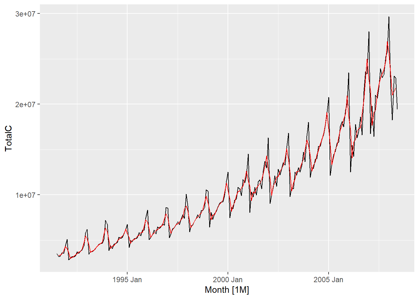
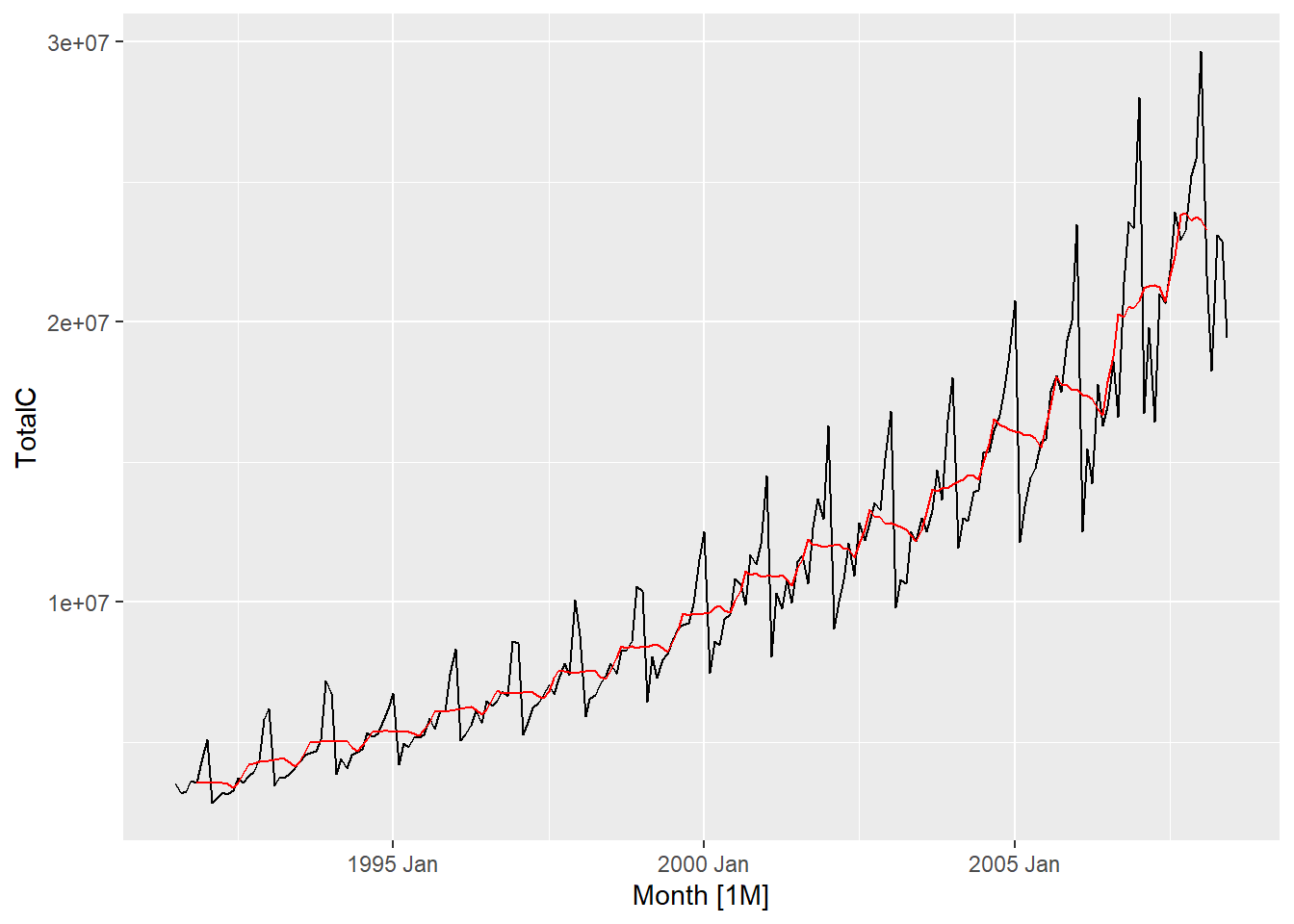
Simple moving averages such as these are usually of an odd order. the middle observation, and \(k\) observations on either side, are averaged. In case of even, moving average to a moving average is applied to make an even-order moving average symmetric. Also, weighted MAs are used to yield a smoother estimate of the trend-cycle.

The classical method of time series decomposition originated in the 1920s and was widely used until the 1950s. It still forms the basis of many time series decomposition methods, so it is important to understand how it works. The first step in a classical decomposition is to use a moving average method to estimate the trend-cycle. A moving average of order \(m\) can be written as

\(T_t = 1/m \sum_{j = -k}^k y_{t+j}\) where \(m = 2k+1\)

The estimate of the trend-cycle at time \(t\) is obtained by averaging values of the time series within \(k\) periods of \(t\) . Observations that are nearby in time are also likely to be close in value. Therefore, the average eliminates some of the randomness in the data, leaving a smooth trend-cycle component. We call this an \(m-MA\), meaning a moving average of order \(m\).

diab_ma5 <- df_diab |>
  mutate(
    `5-MA` = slider::slide_dbl(TotalC, mean,
                .before = 2, 
                .after = 2, 
                .complete = TRUE)
  )

To see what the trend-cycle estimate looks like, we plot it along with the original data

Think over!

How will you calculate moving averages for 3-MA, 7-MA, and 9-MA?

Code

diab_ma3 |>
  autoplot(TotalC) +
  geom_line(aes(y = `3-MA`), colour = "red") 
diab_ma5 |>
  autoplot(TotalC) +
  geom_line(aes(y = `5-MA`), colour = "red") 
diab_ma7 |>
  autoplot(TotalC) +
  geom_line(aes(y = `7-MA`), colour = "red") 
diab_ma9 |>
  autoplot(TotalC) +
  geom_line(aes(y = `9-MA`), colour = "red") 

(a) 3-MA

(b) 5-MA

(c) 7-MA

(d) 9-MA

Figure 3: Moving averages