Mid-workshop Hands-On Exercise

Welcome to the world of Time Series Analysis and forecasting!!

1 Introduction.

There are two hands-on exercises planned for you in this workshop. The first one is on basic starting steps which we will do now and the other is at end of the workshop which is based on workflows. In this exercise, the participants have to follow the principles and practices as explained in the workshop so far. We have to do the following actions for completion of this exercise:

1. Create a new project titled “time_series” at a desired location in the computer.
2. Create folders named “data” and “scripts”.
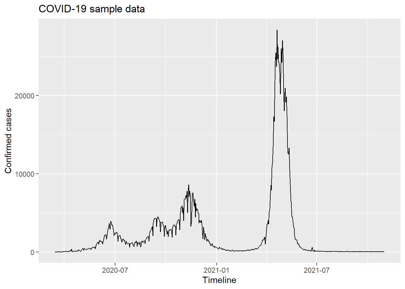
3. Copy the “covid_IPHACON2024.csv” file to the data folder.
4. Create a script and name it as “covid_analysis”.
5. Load libraries.
6. Load data.
7. Explore data
8. Calculate traditional statistics.
9. Create a time series object.

Tip

It is a good practice to always have a new project and dedicated folders for your independent research activities. It enables better database management especially when you are involved in multiple research activities. Project based approach is also helpful in better communication and sharing of the workflows.

2 Load libraries.

Once your project is ready with specified folders and files at right locations, working in modular fashion provides a more intuitive approach to your analysis. Let’s load libraries for working further.

library(tidyverse) 

── Attaching core tidyverse packages ──────────────────────── tidyverse 2.0.0 ──
✔ dplyr     1.1.2     ✔ readr     2.1.4
✔ forcats   1.0.0     ✔ stringr   1.5.0
✔ ggplot2   3.4.2     ✔ tibble    3.2.1
✔ lubridate 1.9.2     ✔ tidyr     1.3.0
✔ purrr     1.0.1     
── Conflicts ────────────────────────────────────────── tidyverse_conflicts() ──
✖ dplyr::filter() masks stats::filter()
✖ dplyr::lag()    masks stats::lag()
ℹ Use the conflicted package (<http://conflicted.r-lib.org/>) to force all conflicts to become errors

library(fpp3)

── Attaching packages ────────────────────────────────────────────── fpp3 0.5 ──
✔ tsibble     1.1.3     ✔ fable       0.3.3
✔ tsibbledata 0.4.1     ✔ fabletools  0.3.3
✔ feasts      0.3.1     
── Conflicts ───────────────────────────────────────────────── fpp3_conflicts ──
✖ lubridate::date()    masks base::date()
✖ dplyr::filter()      masks stats::filter()
✖ tsibble::intersect() masks base::intersect()
✖ tsibble::interval()  masks lubridate::interval()
✖ dplyr::lag()         masks stats::lag()
✖ tsibble::setdiff()   masks base::setdiff()
✖ tsibble::union()     masks base::union()

Loading libraries.

We should be careful in loading libraries. Loading unwarranted libraries and those which are going to be utilised only once or twice in the entire analysis is not a good habit as it unnecessarily burdens the system and compromises computational efficiency!

3 Load data.

df_covid <- rio::import(here::here("data",
                       "covid19_IPHACON2024.csv"))

4 Explore data

Let us glimpse the datatset at the start of analysis. Interpret the results.

df_covid |> 
  glimpse()

Rows: 23,283
Columns: 4
$ Date_YMD <IDate> 2020-03-14, 2020-03-14, 2020-03-14, 2020-03-14, 2020-03-14,…
$ Status   <chr> "Confirmed", "Confirmed", "Confirmed", "Confirmed", "Confirme…
$ name     <chr> "TT", "AN", "AP", "AR", "AS", "BR", "CH", "CT", "DN", "DD", "…
$ value    <int> 81, 0, 1, 0, 0, 0, 0, 0, 0, 0, 7, 0, 0, 14, 0, 2, 0, 6, 19, 0…

4.1 Which states are icluded in the dataset?

df_covid |> 
  select(name) |> 
  mutate(name = factor(name)) |> 
  summary()

      name      
 AN     :  597  
 AP     :  597  
 AR     :  597  
 AS     :  597  
 BR     :  597  
 CH     :  597  
 (Other):19701  

4.2 What is the timeline of the dataset?

df_covid |> 
  select(Date_YMD) |> 
  summary()

    Date_YMD         
 Min.   :2020-03-14  
 1st Qu.:2020-08-10  
 Median :2021-01-06  
 Mean   :2021-01-06  
 3rd Qu.:2021-06-04  
 Max.   :2021-10-31  

4.3 Subset dataset for a state of your choice.

df <- df_covid |> 
  filter(name == "DL")

4.4 What is the total number of cases reported from the state during this period?

df |> 
  summarise(total = sum(value))

    total
1 1439870

4.5 When was maximum number of cases reported from the state?

df |> 
  filter(value == max(value))

    Date_YMD    Status name value
1 2021-04-20 Confirmed   DL 28395

4.6 Draw an epidemic curve for your selected state and interpret.

df |> 
  ggplot() +
  geom_line(aes(Date_YMD, value)) +
  labs(
    title = "COVID-19 sample data",
    x = "Timeline",
    y = "Confirmed cases"
  )

4.7 Convert your dataset into a time series object with weekly timestamp

df <- df |> 
  mutate(Date_YMD = yearweek(Date_YMD)) |> 
  group_by(Date_YMD) |> 
  summarise(value = sum(value)) |> 
  as_tsibble(index = Date_YMD)

Now since we have created a time series object, lets move further.

Further exercises.

During the workshop, as we proceed, we shall be getting back to this exercise for calculating time series features and understanding concepts such as ACF, MAs, etc. Happy learning!