ARIMA models
Welcome to the world of Time Series Analysis and forecasting!!
1 Introduction.
Exponential smoothing and ARIMA models are the two most widely used approaches to time series forecasting, and provide complementary approaches to the problem. While exponential smoothing models are based on a description of the trend and seasonality in the data, ARIMA models aim to describe the autocorrelations in the data.
2 Autoregressive (AR) models.
Autoregressive models are remarkably flexible at handling a wide range of different time series patterns. In an autoregression model, we forecast the variable of interest using a linear combination of past values of the variable. The term autoregression indicates that it is a regression of the variable against itself. Thus, an autoregressive model of order \(p\) can be written as
\(y_t = c + \phi_1 y_{t-1}+ \phi_2y_{t-2}+ \phi_3y_{t-3}+.... \phi_py_{t-p} + \epsilon_t\)
3 Moving average (MA) models.
In case of MA models, rather than using past values of the forecast variable in a regression, past forecast errors are used in a regression-like model
\(y_t = c + \theta_1.\epsilon_{t-1}+ \theta_2.\epsilon_{t-2}+ \theta_3.\epsilon_{t-3}+.... \theta_p. \epsilon_{t-p} + \epsilon_t\)
4 Autoregressive Moving Average models.
A seasonal ARIMA model is formed by including additional seasonal terms in the ARIMA models and are represented as ARIMA(p,d,q)(P,D,Q)m.
If we combine differencing with autoregression and a moving average model, we obtain a non-seasonal ARIMA model. ARIMA is an acronym for AutoRegressive Integrated Moving Average. This is called as ARIMA(\(p,d,q\)) model where \(p\) is the order of AR, \(q\) is the order of MA, and \(q\) is the order of differencing.
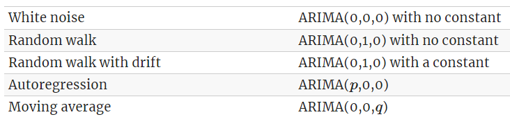
Special cases of ARIMA models